cache memory #
1. Introduction to Cache Memory #
Cache memory is a small, high-speed SRAM buffer positioned between the CPU and main memory (DRAM). Its primary purpose is to bridge the performance gap caused by slow DRAM access speeds.
flowchart LR
CPU["CPU"] <--> MEM["Main Memory"]
-
Performance Gain: Dramatically improves throughput for data and instructions accessed more than once.
-
Access Time: The elapsed time required to transfer data from main memory to the CPU, or write data back from the CPU to main memory.
-
Economic Trade-off: Fast memory (SRAM) is expensive per byte, whereas main memory (DRAM) is cheap but slow. A hierarchical cache system balances both constraints to achieve low average cost and high average speed.
$$\text{Access Time} \propto \frac{1}{\text{Speed}}$$
2. Memory Access Models #
-
Direct Access (No Cache): Without cache, every single memory request travels directly over the system bus to DRAM.
flowchart TD subgraph Direct Access CPU1["CPU"] <--> |"200ns \n byte-addressable"| MEM1["Memory"] end -
Cached Access: With cache enabled, memory requests first check the fast SRAM cache. Transfers between DRAM and cache occur in fixed-size blocks (cache lines).
flowchart TD subgraph Cached Access CPU2["CPU"] <--> |"15ns"| CACHE["Cache"] CACHE <--> |"200ns \n block-based \n (in parallel)"| MEM2["Memory"] end -
Latency Analysis
- First Access (Cache Miss): 200ns +15ns = 215ns (Fetches block into cache and serves CPU).
- Subsequent Accesses (Cache Hit):15ns (Served directly from SRAM).
3. Principle of Locality #
The Principle of Locality is the empirical tendency of a processor to access the same set of memory locations repeatedly over a short period. Caching works efficiently because computer programs naturally exhibit two distinct types of locality:
-
Temporal Locality: If a memory location is referenced once, it is very likely to be referenced again in the near future.
-
Example: Loop control variables, accumulator registers, and repeated function calls.
-
Implementation: When an item is first fetched from main memory, store it in the cache and retain it for a duration.
// Temporal Locality Example:
// The variables 'n', 'swapped', 'i', and 'j' are
// repeatedly accessed in cache throughout execution.
func bubbleSort(arr []int) {
    n := len(arr)
    for i := 0; i < n-1; i++ {
        swapped := false
        for j := 0; j < n-i-1; j++ {
            if arr[j] > arr[j+1] {
                arr[j], arr[j+1] = arr[j+1], arr[j]
                swapped = true
            }
        }
        if !swapped {
            break
        }
    }
}
-
-
Spatial Locality: If a memory location is referenced, nearby memory locations are very likely to be referenced in the near future.
- Sequential instruction execution (program code flow).
- Contiguous data structures (e.g., iterating through an array, vector, or image pixel buffer). During the loop. the array is cached
-
Implementation: When a single memory address is requested, fetch its entire neighboring block (cache line) into the cache simultaneously.
- Block Fetching: Fetching entire blocks (e.g., 64 bytes) rather than single bytes capitalizes on spatial locality.
- Data Retention: Retaining fetched blocks in cache memory over time capitalizes on temporal locality.
Theoretical Overview: Linked List vs. Array #
In high-level data structure design, Linked Lists are often introduced as flexible structures where nodes link dynamically to each other.
Algorithmic Complexity Comparison #
- Insertion/Deletion (Write):
- Linked List: \(O(1)\) time complexity (modifying at most 2-3 node pointers once the position is located).
- Array: \(O(n)\) time complexity in the worst case (requires shifting elements or reallocating to a larger contiguous array block).
- Flexibility:
- Linked List: Dynamic size allocation without needing contiguous memory blocks.
- Array: Fixed-size memory allocation (or costly dynamic resizing overhead).
In pure theoretical time complexity (\(O\)-notation), linked lists appear superior or equal to arrays for dynamic write operations.
Practical Hardware Bottleneck: Pointer Chasing & Cache Efficiency #
- Address Resolution Overhead
- Linked List: Finding the target node requires sequential traversal (pointer chasing), checking memory addresses node-by-node from head to tail.
- Array: Uses a single base address with a calculated byte offset:
- $$\text{Address}(i) = \text{Base Address} + (i \times \text{Element Size})$$
- Memory Latency vs. Write Time
- Traversing main memory to find a node’s physical memory address can be 100x slower than executing the actual pointer modification or write operation in cache/registers.
Impact on Cache Performance #
Hardware cache hierarchies (L1/L2/L3) rely heavily on Spatial Locality (fetching entire contiguous cache blocks of 32-64 bytes from main memory).
| Metric | Array | Linked List |
|---|---|---|
| Memory Layout | Contiguous RAM allocation | Fragmented / Dispersed heap nodes |
| Spatial Locality | High (Sequential elements share cache lines) | Low (Nodes reside across distinct memory lines) |
| Hardware Prefetching | Optimal (CPU prefetcher predicts next indices) | Poor (Pointer addresses cannot be precalculated) |
| Cache Miss Ratio | Very Low | Very High |
- Arrays maximize hardware cache efficiency because consecutive elements reside in the same pre-loaded cache blocks.
- Linked Lists suffer from high cache miss rates due to arbitrary node allocation across heap memory.
- As a result, standard linked lists are generally suitable only for specific restricted use cases (e.g., non-performance-critical dynamic queues or lock-free concurrent node manipulation) where physical memory layout constraints override raw cache throughput.
Cache Design #
1. Core Mechanics: Cache Hits and Misses #
flowchart TD
  subgraph Cached Access
    CPU["CPU"] <--> |"short accessing time"| CACHE["Cache \n (Cache Lines / Blocks)"]
    CACHE <--> |"block-based \n (in parallel)"| MEM2["Main Memory \n (Blocks)" ]
    CPU <--> |"long accessing time"| MEM2
  end
Fundamental Cache Operations #
- When a block copied from memory to cache
- On a Cache Miss: When the CPU requests a memory address that is not currently present in the cache, a cache miss occurs.
- The cache controller fetches the entire 64-byte block containing the requested address from main memory into a cache line to satisfy the request and leverage spatial locality.
- block placed in the cache (Mapping Functions)
- Direct Mapping: Each main memory block maps to exactly one specific cache line: $$\text{Cache Line Index} = (\text{Block Address}) \pmod{\text{Total Cache Lines}}$$
- Fully Associative Mapping: A block can be placed in any available cache line. (Requires parallel tag searching).
- Set-Associative Mapping: Cache is divided into sets. A block maps to a specific set, but can reside in any line within that set (e.g., 2-way, 4-way, 8-way).
- when the mapped location is already occupied (Replacement Algorithms)
- When all candidate cache lines are full, a replacement policy selects which existing block to evict:
- LRU (Least Recently Used): Evicts the line that hasn’t been accessed for the longest time.
- FIFO (First-In, First-Out): Evicts the line that was loaded earliest.
- Random: Randomly selects a line to evict (simple hardware implementation).
- Write Policies for Eviction/Updates:
- Write-Through: Updates both Cache and Main Memory simultaneously.
- Write-Back: Updates only Cache and sets a Dirty Bit. Memory is updated only when the line is evicted.
- When all candidate cache lines are full, a replacement policy selects which existing block to evict:
2. Cache Size Optimization #
Selecting the optimal cache size involves balancing cost, speed, and hit rate:
- Lower Bound (Small Cache): Keeps total system cost per bit close to main memory, but increases cache misses.
- Upper Bound (Large Cache): Maximizes hit rates, but increases hardware costs and can slightly increase access latency due to larger, complex address decoding logic.
- Typical Capacity Range: Historically 1 KB to 512 KB per core in legacy systems; modern L1/L2 caches range from 32 KB to 2 MB per core, with shared L3 caches reaching tens of megabytes.
cache Trade-offsParameter Trend Explanation Cache Hit Rate $$\uparrow$$ Larger capacity accommodates larger working sets with fewer capacity misses. Manufacturing Cost $$\uparrow$$ occupies significant silicon die area. Hardware Access Latency $$\uparrow$$ Larger memory arrays increase fan-out capacitance and gate delay during address decoding. Cost-to-Performance Ratio $$\approx$$ Beyond a certain size, hit rate gains flatten out while SRAM costs scale linearly with area.
3. Cost Analysis Formulas #
Average Memory Cost per Bit #
The effective cost per bit of a hierarchical memory system is defined as:
$$C_{\text{system}} = \frac{(C_{\text{cache}} \times S_{\text{cache}}) + (C_{\text{main}} \times S_{\text{main}})}{S_{\text{cache}} + S_{\text{main}}}$$- cache,main = Cost per bit of Cache (SRAM) and Main Memory (DRAM).
- cache, main = Storage capacity in bits
Average Access Time (avg) #
$$T_{\text{avg}} = H \cdot T_{\text{cache}} + (1 - H) \cdot (T_{\text{cache}} + T_{\text{penalty}})$$- H = Hit Ratio ( 0 to 1 ).
- cache = Cache hit time (e.g., 15ns).
- penalty = Memory fetch time (e.g., 200ns).
Direct-Mapped Cache Architecture #
In direct mapping, memory block j maps to cache line i according to the modulo function:
$$i = j \bmod m$$- i = Cache line number
- j = Main Memory block number
- m = Total number of lines in cache
Memory Access Latency Hierarchy #
flowchart TD
  subgraph "Cached Access Latency"
    CPU2["CPU"] <--> |"15 ns"| CACHE["Cache Memory\n(0–127 Blocks / Lines)"]
    CACHE <--> |"200 ns\n(Block Transfer)"| MEM2["Main Memory\n(0–4095 Blocks)"]
  end
Architectural Calculations & System Specs #
Given the specifications from your notes:
- Cache to Main Memory Ratio: $$128 : 4096 = 1 : 32$$
- Block Size: $$16\text{ words} (32\text{ bytes}, word-addressable)$$
- Main Memory Size: $$4096\text{ blocks} \times 16\text{ words/block} = 64\text{K words} = 128\text{ KB}$$
- Address Space: $$64\text{K words} = 2^{16} \implies \mathbf{16\text{-bit memory address}}$$
Address Field Breakdown #
The 16-bit physical memory address is divided into Tag, Block (Index), and Word (Offset) fields:
flowchart LR
  tag["Tag\n5 Bits\nIdentifies which of the 32 MM blocks is stored"]
  block["Block / Index\n7 Bits\nLocates the line in cache (0–127)"]
  word["Word / Offset\n4 Bits\nLocates specific word in block (0–15)"]

  tag --- block --- word
- Word Offset (4 bits): Selects one of the 16 words per block (2^4 = 16).
- Block Index (7 bits): Selects one of the 128 cache lines (2^7 = 128).
- Tag Field (5 bits): Identifies which of the 32 mapping blocks (2^5 = 32) occupies the line.
Word Index Breakdown #
Within each block, the 4-bit word field specifies the exact target word offset 0-15:
flowchart TD
  subgraph WordOffset["Word Field Bits (0–15)"]
    A["0000 -> Word 0"]
    B["0001 -> Word 1"]
    C["..."]
    D["1110 -> Word 14"]
    E["1111 -> Word 15"]
  end
Address Mapping Examples #
Using the mapping formula i = j \bmod 128:
Tag Field (5b) |
Block Field (7b) |
Cache Line | Main Memory (MM) Block |
|---|---|---|---|
00000 |
0000000 |
Line 0 | Block 0 $$0 \bmod 128 = 0$$ |
00001 |
0000000 |
Line 0 | Block 128 $$128 \bmod 128 = 0$$ |
00010 |
0000000 |
Line 0 | Block 256 $$256 \bmod 128 = 0$$ |
Key Takeaway: Blocks 0, 128, 256, and all multiples of 128 share the exact same Block Index (0000000₂). They all contend for Cache Line 0, differentiated solely by their Tag value (00000₂, 00001₂, 00010₂).
Direct Mapping Concept #
In a Direct-Mapped cache, each main memory block maps to exactly one specific cache line determined by:
$$\text{Cache Line} = (\text{Main Memory Block Number}) \bmod (\text{Total Cache Lines})$$
flowchart LR
  subgraph DirectMapping["Direct Mapping"]
    cache["Cache Line 0"]

    subgraph MainMemory["Main Memory"]
      block0["Block 0"]
      block128["Block 128"]
      block256["Block 256"]
    end

    cache <--- block0
    cache <--- block128
    cache <--- block256
  end
Memory Address Breakdown #
For a Direct-Mapped system, a physical memory address issued by the CPU is divided into three distinct fields:
| Tag Bits | Block / Index Bits | Word / Offset Bits |
|---|---|---|
| Identifies the specific block owner | Selects the target cache line | Pinpoints the word inside the block |
Step-by-Step Example: Accessing Address 1D00H
#
1. Hexadecimal to Binary Conversion #
The CPU requests memory address 1D00H:
| Hex | 1 | D | 0 | 0 |
|---|---|---|---|---|
| Binary | 0001 |
1101 |
0000 |
0000 |
2. Field Splitting #
Dividing the 16-bit binary string 0001 1101 0000 0000₂ into Tag, Block (Index), and Word (Offset):
| Field | Tag | Block (Index) | Word (Offset) |
|---|---|---|---|
| Binary Value | 00011 |
1010000 |
0000 |
| Hex | 3H |
50H |
0H |
| Decimal | $$3_{10}$$ | $$80_{10}$$ | $$0_{10}$$ |
3. Cache Lookup Execution Path #
- Locate Line: The CPU inspects Block/Line 80 (50H) in the cache.
- Compare Tag: The CPU checks the Tag store for Line 80 against the requested tag (
3H).
- Cache Hit: If
Tag == 3Hand the line is valid, return data immediately from cache Line 80. - Cache Miss: If
Tag != 3H(or line is invalid), copy Block 50H from Main Memory into Cache Line 80, update the Tag field to3H, and supply the word to the CPU.
Direct Mapping:Trade-offs & Limitations #
Advantages #
- Simple Implementation: Low hardware cost and minimal lookup overhead.
- Fast Hit Time: Direct index lookup without parallel tag searches.
Disadvantages #
- Inflexible Placement: Every block has only one valid cache slot.
- Cache Contention (Thrashing): If a program repeatedly accesses two distinct main memory blocks that map to the same cache line, they will continuously overwrite each other.
Example: Thrashing / Contention Loop #
Consider a loop alternating between accesses to blocks:
$$0 \rightarrow 128 \rightarrow 0 \rightarrow 128$$| Main Memory Block | Target Cache Line | Resulting Behavior |
|---|---|---|
| Block 0 | Line 0 | Maps to Line 0 |
| Block 128 | Line 0 | Overwrites Block 0 in Line 0 |
| Block 1 | Line 1 | Maps to Line 1 |
| Block 129 | Line 1 | Overwrites Block 1 in Line 1 |
Impact: Continuous ping-ponging causes a high stream of Cache Misses (thrashing), defeating the purpose of the cache system.
Fully Assoicative #
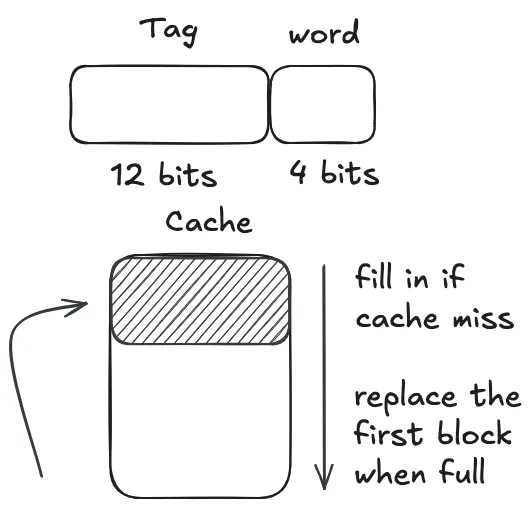
In a Fully Associative Cache, any main memory block can be stored in any cache location.
Search Overhead #
Because there is no index bit restricting placement, the cache hardware must search every single cache line simultaneously using tag comparators:
- Search Cost: High circuit complexity and energy consumption.
- Cache Hit (Avg Search): ~64 blocks searched on average (for a 128-block cache).
- Cache Miss: Must search all 128 blocks to confirm data is absent.
Solution: K-Way Set-Associative Cache #
Set-associative caching provides a optimal trade-off between Direct-Mapped (zero placement flexibility, high contention) and Fully Associative (complete flexibility, high hardware search cost).
Address Format Breakdown #
A single memory address is divided into three fields:
| Field | Description |
|---|---|
| Tag | Identifies the memory block within the set |
| Set Index | Selects the specific set (v = m / K) |
| Word Offset | Locates the word within the block |
2-Way Set-Associative Structure #
For a cache with 128 lines divided into 2-Way Sets:
- Total Lines: 128
- Lines per Set: K = 2 ways
- Number of Sets: v = 128 / 2 = 64 sets (6 bits required for set index)
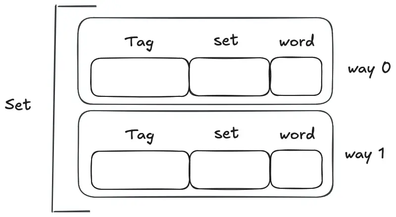
The most common associative configurations in modern processors are 4-way and 8-way set-associative caches, striking an ideal balance between low hit times, reduced tag comparator hardware, and minimal cache thrashing.
Fundamental Relationships & Mapping #
The organization of set-associative cache is defined by two core formulas:
$$m = v \times k$$$$i = j \bmod v$$Where:
- m = Total number of cache lines/blocks (512)
- k = Number of ways per set (2)
- v = Total number of sets
- i = Target cache set index
- j = Main memory block number
Calculating Total Sets (v) #
$$v = \frac{m}{k} = \frac{512}{2} = 256\text{ sets} = 2^8$$Since v = 256, the set mapping function simplifies to:
32-Bit Memory Address Breakdown #
A physical 32-bit address issued by the CPU is partitioned into three functional fields:
| Field | Bit Length | Calculation | Function |
|---|---|---|---|
| Tag | $$20\text{ bits}$$ | $$32 - 8 - 4 = 20\text{ bits}$$ | Uniquely identifies the block stored in a way |
| Set Index | $$8\text{ bits}$$ | $$2^8 = 256\text{ sets}$$ | Selects 1 of the 256 target sets (0-255) |
| Byte Offset | $$4\text{ bits}$$ | $$2^4 = 16\text{ bytes}$$ | Pinpoints 1 of the 16 bytes within a block |
Set Associativity Trade-offs #
A 2-way (or 4-way) set-associative cache provides two (or four) parallel block buffers per set for storing incoming memory blocks.
Fewer Ways (e.g., Direct-Mapped / 1-Way): Lower circuit complexity, lower power consumption, faster hit evaluation, but higher cache conflict misses.
More Ways (e.g., 4-Way / 8-Way): Higher hit rate and reduced thrashing, but increased hardware complexity (more comparators operating in parallel) and slightly longer lookup latency.
Replacement Algorithms #
When a new block, one of the existing blocks must be replaced. direct mapped: must replace Fully associative and set associative: need an replacement algorithm.
- highly affects the system preformance
- Keep blocks in the cache when referenced shortly
Overview of Cache Replacement Policies #
When a cache miss occurs and all target cache lines/ways are occupied, an existing block must be evicted to make space for the incoming block:
- Direct-Mapped Cache: No algorithm needed. Every block maps strictly to 1 cache line (i = j mod m), so an incoming block must replace whatever is currently in that designated line.
- Fully Associative & Set-Associative Caches: Replacement algorithms required. Because a block can reside in multiple lines/ways, an eviction policy decides which block to replace.
- System Impact: Replacement policy efficiency directly dictates hit rates and overall system memory performance.
- Core Goal: Exploit temporal locality—retain blocks in cache that are likely to be referenced again in the near future.
Least Recently Used (LRU) Algorithm #
The LRU strategy replaces the block within the set that has gone the longest duration without being referenced.
2-Way Set-Associative LRU Tracking (1-Bit Implementation) #
In a 2-way set-associative cache (k = 2), LRU tracking can be implemented with a single LRU/Use Bit per way:
- Access Event: Whenever a way in a set is referenced (read/written), its tracking bit is set to
1, while the opposite way’s bit is set to0. - Eviction Event: Upon a cache miss where both ways are valid (
V = 1), the cache evicts data from the way whose tracking bit is0(the least recently used block).
Hardware Scaling (K-Way LRU) #
- For up to an 8-way set-associative cache, a 3-bit counter per line is sufficient to maintain full LRU order tracking, providing an optimal hardware-to-performance trade-off.
Worked Architecture Example: 8-Bit Address System #
System Parameters & Calculations #
- Memory Address Space: 8 bits (Byte-Addressable)
- Main Memory Size: 2^8 bytes = 256 bytes (32 blocks), indexed 0 to 31
- Block Size: 2^3 bytes = 8 bytes (3 bits for byte offset)
- Cache Capacity: 2 x 2^2 blocks = 8 blocks = 64 bytes
- Number of Ways (k): 2
- Number of Sets (v): Total Blocks Ways = 8/2 = 4 sets = 2^2 (2 bits for set index)
Address Format Breakdown #
A physical 8-bit address is partitioned as follows:
| Field | Bit Length | Function |
|---|---|---|
| Tag | 3 bits | Uniquely identifies block within the set (8 - 2 - 3 = 3) |
| Set Index | 2 bits | Selects target set (0–3) |
| Byte Offset | 3 bits | Selects target byte within the 8-byte block (0–7) |
flowchart LR
    Address["8-Bit Physical Address"] --> Tag["Tag\n(3 Bits)"]
    Address --> Set["Set Index\n(2 Bits)"]
    Address --> Byte["Byte Offset\n(3 Bits)"]
Cache Line Entry Structure #
Each line entry within a set contains control flags, tag bits, and the raw data payload:

- Valid Bit (V):
- 0 = Line is empty/invalid (occurs at system power-up; replaced first on a miss).
- 1 = Line holds valid data.
- Dirty Bit (W):
- 0 = Data in cache matches main memory (Clean).
- 1 = Data modified in cache; requires write-back sync before replacement (Dirty).
Initial System State
At power-up, all lines have Valid Bit (V = 0). Any initial access results in a cold miss and populates empty ways top-down before triggering LRU evictions.
other algorithms #
- First-in/first-out (FIFO)
- Least frequently used (LFU)
- Random
Cache Read Architectures #
Cache read operations depend on whether the system accesses memory serially or in parallel.
1. Non-Look-Through (Look-Aside / Parallel Architecture) #
In a standard non-look-through arrangement, the cache and main memory hardware checks occur in sequence.
Cache Hit (15 ns) #
Data is retrieved directly from the cache buffer:
flowchart RL
    subgraph hit ["Cache Hit (15ns): Standard"]
        direction RL
        cache["Cache"] --> hardware1["Hardware Circuit\n(15ns)"] --> cpu["CPU"]
    end
Cache Miss (215 ns) #
The cache check fails first (15 ns), then main memory is accessed to load the requested block into cache (200 ns):
flowchart RL
    subgraph miss ["Cache Miss (215ns): Standard"]
        direction RL
        ram["Main Memory"] --> hardware2["Hardware Circuit\n(200ns)"] --> cache["Cache"] --> hardware1["Hardware Circuit\n(15ns)"] --> cpu["CPU"]
    end
2. Look-Through (Look-Aside Concurrent Read) #
Main memory and cache requests are triggered concurrently.
Cache Hit (15 ns) #
The cache delivers the requested byte faster than memory can respond, so the memory access is aborted:
flowchart RL
    subgraph look_hit ["Cache Hit (15ns): Look-Through"]
        direction RL
        cache["Cache"] --> hardware["Hardware Circuit\n(15ns)"] --> cpu["CPU"]
    end
Cache Miss (200 ns) #
Because the main memory fetch was initiated simultaneously with the cache check, the CPU receives data directly from memory in 200 ns instead of waiting 15 ns + 200 ns:
flowchart RL
    subgraph look_miss ["Cache Miss (200ns): Look-Through"]
        direction RL
        ram["Main Memory"] -->|"200ns Direct Access"| cpu["CPU"]
        ram --> hardware2["Hardware Circuit\n(200ns)"] --> cache["Cache"] --> hardware1["Hardware Circuit\n(15ns)"] --> cpu
    end
- Pro: Faster recovery time on cache misses (200 ns vs 215 ns).
- Con: Requires additional hardware bus control circuitry to manage concurrent memory bus requests.
Cache Write Policies #
When the CPU issues a write operation, the policy dictates how memory consistency is maintained between the cache and main memory.
1. Write-Through #
Every write operation updates both the cache and main memory simultaneously.
flowchart LR
    subgraph write_through ["Write-Through Policy"]
        direction LR
        cpu["CPU"] --> hardware1["Hardware Circuit"] -->|"40ns"| cache["Cache"]
        cpu --> hardware2["Hardware Circuit"] -->|"300ns"| memory["Main Memory"]
    end
- Pros: Main memory is always up-to-date; simple hardware implementation.
- Cons: Write speed is bounded by slow main memory write latency (300 ns).
2. Write-Back (Deferred Write) #
The CPU writes updated data only to the cache. Main memory is updated later only when the modified block is evicted to make room for a new block.
flowchart LR
    subgraph write_back ["Write-Back Policy"]
        direction LR
        cpu["CPU"] --> hardware1["Hardware Circuit"] -->|"40ns"| cache["Cache"]
        cache --> hardware2["Hardware Circuit\n(Eviction Sync)"] -->|"300ns (If Dirty)"| memory["Main Memory"]
    end
- Dirty Bit (Write Bit): Set to
1whenever a cache block is modified. When evicted, ifDirty = 1, the line is written back to main memory; ifDirty = 0, it is simply overwritten. - Trade-off: Increases algorithm & hardware complexity (tracking dirty bits/evictions) to significantly reduce the frequency of slow main memory updates.
Write Miss Policies #
What happens when a CPU attempts to write to an address that is not currently in the cache?
1. Write Allocate (Fetch-on-Write) #
The block containing the target address is loaded from main memory into the cache, and then updated in the cache.
flowchart LR
    subgraph write_alloc ["Write Allocate"]
        direction LR
        cpu["CPU"] --> hardware1["Hardware Circuit"] --> cache["Cache"]
        cache --> hardware2["Hardware Circuit\n(Sync if Evicted)"] --> memory["Main Memory"]
    end
- Typically paired with Write-Back policies.
2. Write No-Allocate (No-Fetch-on-Write) #
The write operation bypasses the cache entirely and modifies main memory directly. The block is not brought into cache.
flowchart LR
    subgraph write_no_alloc ["Write No-Allocate"]
        direction LR
        cpu["CPU"] --> hardware1["Hardware Circuit"] --> memory["Main Memory\n(Bypass Cache)"]
    end
- Typically paired with Write-Through policies.
Cache Line (Block) Size vs. Hit Ratio #
Selecting an appropriate cache block size requires balancing spatial locality benefits against available cache line capacity and transfer overhead.
1. Too Small Line Size #
- Pros: Maximizes the total number of distinct lines/blocks available in the cache, which reduces conflict misses for scattered memory access patterns.
- Cons: Lowers the spatial locality benefit because neighboring bytes are not prefetched together in a single transfer.
2. Optimal Line Size #
- Pros: Increases the overall Hit Ratio by exploiting Spatial Locality (since execution threads frequently access sequential memory locations).
- Cons: Provides fewer total cache blocks for a fixed total cache capacity.
3. Excessively Large Line Size #
- Decreased Hit Ratio: As block size becomes too large relative to total cache capacity, the total number of available lines drops significantly, forcing frequent evictions.
- Cache Pollution: Words loaded inside a massive block may never be referenced by the CPU, wasting memory bus bandwidth and precious cache footprint.
- Higher Miss Penalty: Transferring oversized blocks across the system bus requires significantly more bus cycles per miss.
Single Cache vs. Multiple Caches #
Single Cache: A single unified cache structure used for both instructions and data.
- Pros: High hit rate for simple workloads and straightforward hardware implementation.
- Cons: Creates resource contention between instruction fetching and data execution accesses.
Multiple Caches (Split I/D Caches):
- Contention Elimination: Separating into an Instruction Cache (I-Cache) and a Data Cache (D-Cache) eliminates access contention between the instruction fetch unit and the execution unit.
- Pipeline Efficiency: Essential for hardware pipelining, allowing simultaneous instruction fetching and data load/store operations within the same clock cycle.
- DMA Interactivity: Helps isolate core cache activity when Direct Memory Access (DMA) controllers read or write to main memory independently.
Key Performance Indicators #
Evaluating cache system performance relies on measuring how frequently requests are satisfied by the cache versus how long total memory accesses take.
1. Hit Ratio (HR) #
The fraction of total memory accesses that are successfully found in the cache.
$$HR = \frac{\text{Number of Cache Hits}}{\text{Total Memory Accesses}}$$The HR should around 90% generally.
2. Miss Ratio (MR) #
The fraction of total memory accesses that are not found in the cache, requiring a main memory lookup.
$$MR = \frac{\text{Number of Cache Misses}}{\text{Total Memory Accesses}} = 1 - HR$$Effective Access Time (EAT) #
Effective Access Time (EAT) represents the average time required for the CPU to access a word in the memory hierarchy, factoring in both hits and misses.
1. Non-Look-Through (Look-Aside / Sequential Read) #
In a standard sequential architecture, a cache miss incurs the cache lookup latency (T_c) plus the main memory penalty (T_m).
$$EAT = HR \times T_c + (1 - HR) \times (T_c + T_m)$$Simplifying the equation:
$$EAT = T_c + (1 - HR) \times T_m$$Where:
- $$T_c = \text{Cache Access Latency}$$
- $$T_m = \text{Main Memory Access Latency}$$
- $$1 - HR = \text{Miss Ratio } (MR)$$
2. Look-Through (Concurrent Read) #
In a concurrent look-through architecture, main memory lookup is initiated simultaneously with the cache check. On a miss, the penalty is simply T_m (since main memory was already fetching in parallel).
$$EAT = HR \times T_c + (1 - HR) \times T_m$$Pipelining #
Pipelining is a fundamental hardware optimization technique that enables multiple instructions to execute concurrently in an assembly-line fashion.
- Stage Separation: The overall execution path of an instruction is divided into distinct operational stages (e.g., Instruction Fetch, Decode, Execute, Memory Access, Write Back).
- Dedicated Hardware: Each stage is backed by specialized hardware registers and execution units.
- Overlapped Execution: Successive operations start, execute, and complete sequentially, overlapping in time across different hardware stages.
flowchart LR
    subgraph Pipe ["4-Stage Pipeline Execution"]
        direction LR
        IF["Instruction Fetch (IF)"] --> ID["Instruction Decode (ID)"] --> EX["Execute (EX)"] --> WB["Write Back (WB)"]
    end
Execution Time Comparison & Speedup #
When evaluating execution performance, single-task completion latency differs from overall throughput:
T_s: Time required to complete a single process in serial execution (non-pipelined).T_p: Time required to complete a single process in pipelined execution.
Latency Relationship #
- Ideal Case: T_s == T_p (Assuming pipeline register overhead and stage synchronization delays are zero).
- Real-World Case: T_s <= T_p (Pipeline register clocking, latch delays, and unbalanced stage lengths make the single-task latency slightly higher in a pipelined system).
Speedup Ratio (S) #
The Speedup Ratio (S) measures the performance gain achieved by transitioning from a non-pipelined architecture to a pipelined architecture for a task stream:
$$S = \frac{T_{\text{Non-Pipelined}}}{T_{\text{Pipelined}}}$$For an k-stage pipeline executing n instructions with stage delay τ:
$$S = \frac{n \times k \times \tau}{(k + n - 1) \times \tau} = \frac{n \times k}{k + n - 1}$$As the number of instructions n becomes very large (n - infinity), the maximum theoretical speedup approaches the number of pipeline stages (k):
$$\lim_{n \to \infty} S = k$$The Branch Hazard Problem #
Control hazards caused by conditional branch instructions significantly degrade pipeline execution efficiency:
When a conditional branch is fetched, the CPU does not know the next target address until the branch condition is evaluated in a later stage (e.g., Execution stage). Fetching incorrect subsequent instructions leads to pipeline stalls and wasted cycles.
Fixes & Mitigation Strategies #
To maintain high throughput in the presence of conditional branches, processors employ specialized branch resolution architectures:
Solution 1: Branch Prediction & Speculative Execution #
- Branch Prediction: The CPU guesses whether a conditional branch will be taken or not taken based on past history (dynamic branch predictor) or branch direction heuristics (static branch predictor).
- Correct Guess: The pipeline operates at full speed without stalling (Gain).
- Incorrect Guess: The speculatively fetched instructions are flushed, and the pipeline re-fetches from the correct target address (Misprediction Penalty).
- Speculative Execution: The CPU executes instructions along the predicted path before the branch condition is calculated with certainty. Results are held in speculative registers and committed only when confirmed correct.
Solution 2: Simultaneous Execution of Both Paths (Dual-Path Fetch) #
- Concept: Instead of guessing one path, the CPU fetches and decodes instructions from both the branch target path and the sequential path concurrently.
- Resolution: Once the conditional branch condition is finally evaluated, execution on the incorrect path is aborted, and hardware resources focus entirely on the correct path.
- Constraint: Requires duplicate instruction fetch hardware and execution units, so it can only be implemented when system hardware resources permit.
While multi-path execution guarantees zero branch misprediction latency, modern high-performance processors predominantly use advanced Branch Prediction with Speculative Execution (achieving >95% accuracy) due to reduce hardware resource overhead.